Authors: V. Niarchos, C. Papageorgakis, P. Richmond, A. G. Stapleton, M. Woolley
Paper available on the arXiv at 2306.15730. Included as reference [1]
Abstract
We study the conformal bootstrap of 1D CFTs on the straight Maldacena–Wilson line in 4D \({\cal N}=4\) super-Yang–Mills theory. We introduce an improved truncation scheme with an ‘OPE tail’ approximation and use it to reproduce the ‘bootstrability’ results of Cavaglià et al. for the OPE-coefficients squared of the first three unprotected operators. For example, for the lowest-dimension OPE-coefficient squared at ‘t Hooft coupling \((4\pi)^2\), linear-functional methods with two sum rules from integrated correlators give the rigorous result \(0.294014873 \pm 4.88 \cdot 10^{-8}\), whereas our methods give with machine-precision computations \(0.294014228 \pm 6.77 \cdot 10^{-7}\). For our numerical searches, we benchmark the Reinforcement Learning Soft Actor-Critic algorithm against an Interior Point Method algorithm (IPOPT) and comment on the merits of each algorithm.
How our results compare:
Unconstrained Soft-Actor-Critic and IPOPT
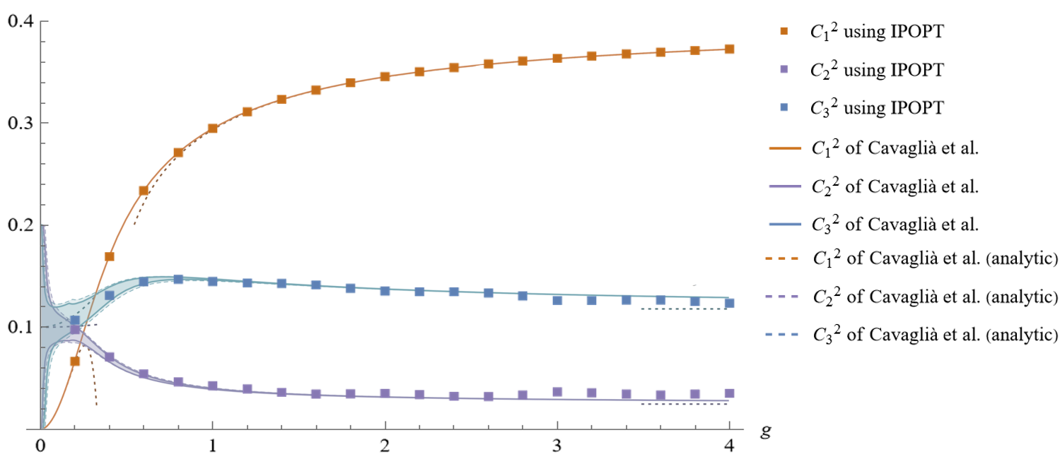
 Results for the OPE-coefficients squared of the first three long operators with no integral constraints. The solid lines indicate the rigorous bounds presented in Figure 6 of [2], reprinted here with permission from the authors. Same-coloured circles and squares indicate our results from the SAC and IPOPT runs respectively. The corresponding statistical errors are too small to display on this plot but can be found in Table 7 of [1].
Constrained Interior Point Optimiser (IPOPT)
 Results for the OPE-coefficients squared of the first three long operators after the incorporation of two integral constraints. The solid lines indicate the rigorous bounds presented in Figure 10 of [3], reprinted here with permission from the authors. Same-colored squares indicate our results from the IPOPT runs. The corresponding statistical errors are too small to display on this plot but can be found in Table 7 of [1]
References
- [1] V. Niarchos, C. Papageorgakis, P. Richmond, A. G. Stapleton and M. Wooley,
Bootstrability in Line-Defect CFT with Improved Truncation Methods, arXiv:2306.15730
- [2] A. Cavaglià, N. Gromov, J. Julius & M. Preti
Integrability and conformal bootstrap: One dimensional defect conformal field theory,
Phys. Rev. D 105, L021902 (2022), arXiv:2107.08510
- [3] A. Cavaglià, N. Gromov, J. Julius & M. Preti
Bootstrability in defect CFT: integrated correlators and sharper bounds,
JHEP 2205, 164 (2022, L021902 (2022), arXiv:2203.09556